Binomial Option Pricing

In my previous post I bought a CBOE dataset and calculated the implied volatility of AAPL calls across strike price, time to expiration, moneyness, and more. To get implied volatility from price I used the Black-Scholes model, which assumes, among many things, that dividends are continuous and that the option can only be exercised at expiration.

For my dataset, historic (2018) AAPL calls and puts, these assumptions definitely aren't accurate. Luckily, we can use a binomial pricing model to look at implied volatility through a different angle.

I decided to use the Cox-Ross-Rubenstein model, which I implemented in Python straight from their 1979 paper. How does it work?

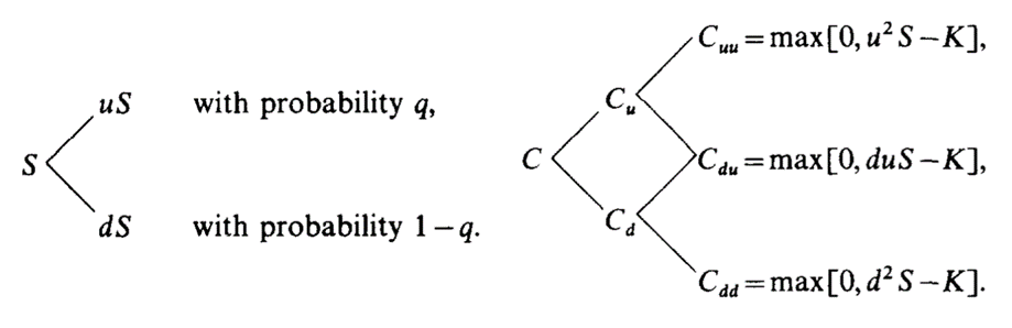
The Cox-Ross-Rubenstein model assumes that at small discrete time steps, the price of the underlying security can either move down a proportion d or up a proportion u, with probability p and (1 - p). If we plot this across many time steps, we can build a binomial tree, where each node is the price of the underlying security at that time step. We can then very easily calculate the hypothetical price of an option at each ending node:



I'm going to skip past most of the math, but the model's fundamental premise is that price of a call or put can be modeled by constructing a hypothetical hedging portfolio and assuming that there can be no risk-free profits to be made by arbitraging between them. (The original paper has a very lucid discussion of this.)

Cox, Ross, and Rubenstein go on to put p in terms of u, d, and the interest rate. Then they show that the values of u and d can be put in terms of volatility and time-to-expiry, and that in the limiting case where the number of steps in a time interval approaches infinity, their binomial model converges to the Black-Scholes model itself!

This is what the crux of the Cox-Ross-Rubenstein pricing formula looks like:



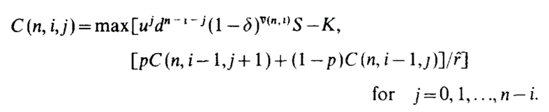
I won't explain it in detail, but essentially it does three things: it makes a binomial tree whose nodes are the prices of the underlying, it finds the hypothetical price of an option at each possible ending node, and it works recursively from each pair of ending nodes to find the price of their parent node, and so on until it reaches the initial node.

Looks like we won't be able to solve it analytically for implied volatility. What's more, the Cox-Ross-Rubenstein formula is very numerically intensive, and we won't be able to find a derivative in order to use the Newton-Raphson method to find implied volatility like we did last time.

Thankfully, we can use the same datasets as last time for option data, underlying data, and interest rate data.

Unfortunately, the same process we used for Black-Scholes, with mostly vanilla Python and a lot of loops, won't cut it here. Cox-Ross-Rubenstein is very intensive and we'll need to optimize a lot. Because a lot of the NumPy library's procedures are precompliled in C++ with Python functioning only as a wrapper, we'll be able to save a lot of time by vectorizing as many things as possible to bypass vanilla Python.

(Thus begins our quest to expunge the scourge of the sluggish and odious for-loop.)

The first challenge was to implement Cox-Ross-Rubenstein itself. As you can see from the formula above, it's not only complex and heavily recursive, it also has a for-loop built right in. When I first saw the formula, I barely knew how to implement it, let alone how to optimize it to run on a large dataset.

The first thing I realized I had to do, was split up the recursive and non-recursive parts. I didn't see a way around the recursion, but as long as I kept the algorithm lean enough and the number of steps n small enough, everything could still work.

To begin with, I had to make a tree containing every possible price of the underlying; to do this, I had to figure out how to represent it. My first instinct was to make a binary tree, until I realized during the implementation that there would be a lot of wasted space. A binary tree grows like 2ⁿ but a binomial tree, like Pascal's Triangle (or Cox-Ross-Rubenstein), grows like 1 + 2 + 3 + ... + n. I would represent this in the most compact form possible, a one-dimensional array.

But a binary tree's node's children's indices could be accessed easily with the formula 2i + 1 and 2i + 2 for the left and right child, respectively. I didn't know a simple formula like that for a binomial tree, and the visible solutions on the internet all involved matrices, loops, or multiple arrays (this wasn't a very popular problem).

Moreover, even if I could find a way to find a child's index from its parent's index, I would still need a way to determine its depth and its path, just from the index! (Unlike a matrix, a 1D array has no row or column.) So fundamentally, any node's index, a single predetermined value, would have to encode two other values. I tried a number of approaches, including representing nodes as strings ['0','U','D','UU','UD','DD'...] and multiplying depth by a large base and adding it to path (dp = depth*1000 + path; depth = dp // 1000; path = dp % 1000), but all of these were too complicated or too difficult to reverse. The best solution turned out to be Cantor's pairing function (the only quadratic method of mapping two numbers onto one):



But I was still stuck. Cantor's pairing function seemed like another overcomplicated procedure to heap onto my teetering mess of an array. Even if it worked, I still wouldn't have a good way to traverse the tree: I might know the position of a node from its index, but what about the indices or positions of its children?

I was about to give up and implement the binomial tree as a triangular matrix.

That was when, staring numbly at the Wikipedia page for pairing functions in the small hours of the morning, I finally saw it:



...It was a triangle. A triangle! Ok, not that triangle. But still.

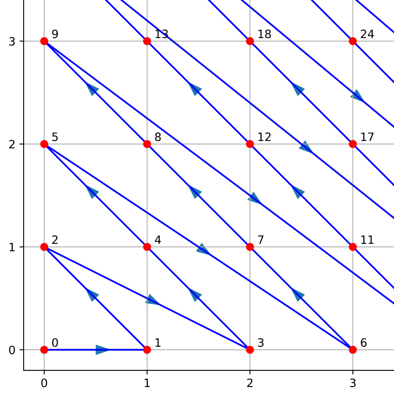
Suddenly I knew what I had to do. A triangle was basically a binomial tree, right? Like with Pascal's Triangle. And if you rotated the triangle formed by Cantor's pairing function, you not only had the fascimile of a tree, you also had the perfect order in which to arrange it, with no need for fancy tricks! It was naturally a breadth-sorted binomial tree!

It didn't take long before I also had a way of traversing the tree algebraically (start at zero and keep a counter i = 1, which increments each time you travel. If j is the node you are currently on, the left child is [i+j+1] and the right child is [i+j].)

Coding the recursive part was very straightforward, and now my pricing function was complete.

This left only the root-finding part. Optimizing this was very tricky; because I recursion was unavoidable, I absolutely needed a method that would converge as quickly as possible. I also didn't know what a graph of Cox-Ross-Rubenstein looked like, especially with so many possible inputs, so the order of convergence also had to be very consistent. These two constraints meant that most of the older methods, such as the bisection, secant, and regula falsi methods, were out.

In the end I received an enormous stroke of luck. Just a few weeks ago, in December 2020, the researchers Oliveira and Takahashi, in the paper linked here, published the first ever root-finding algorithm which strictly improved on the bisection method, preserving its worst-case reliability while achieving superlinear convergence! I couldn't have asked for better timing.

When I adapted their method to my Cox-Ross-Rubenstein pricing model, the function converged to find the implied volatility with a mean of ~6 steps and a max of 22. (I set the upper and lower bounds to 0 and 5, and the error threshold to 0.0001.)

Vectorizing my original program was also fairly straightforward. Performance improved dramatically; on my 2015 laptop with no GPU, it took 0.8 seconds for a single data point, 1.2 seconds for 44 data points, 18 seconds for 500 data points, 130 seconds for 5,000 data points, and 710 seconds for 25,000 data points. (Not tested rigorously, and I had many other applications open while I was waiting for the calculations.)

So, let's take a look at the data!

First, a small collection of at-the-money calls.



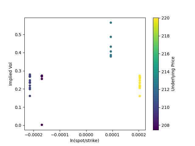
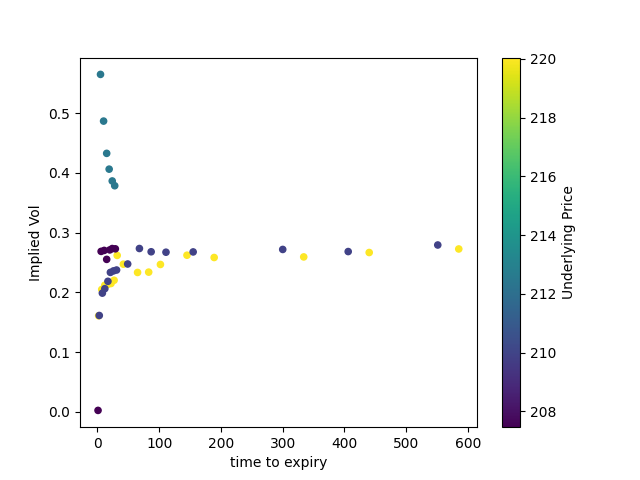
We can see that they cluster roughly by quote date (which we can see by the changing price of the underlying). And we can already see how implied volatility gets much wider as options trade closer to expiration.

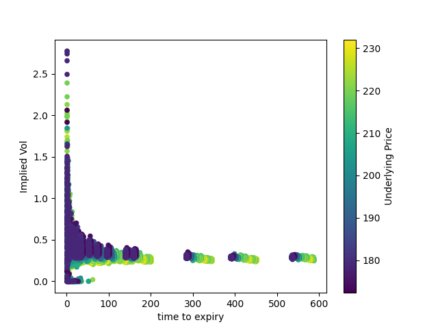
Now for ~500 data points which are still roughly at-the-money:



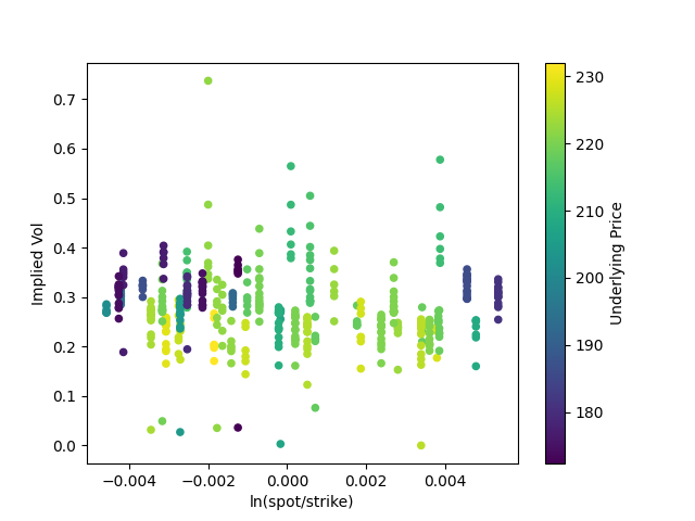
Much of the same. It's also fairly similar to our results from Black-Scholes.

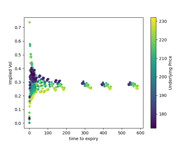
Here are some of the middle values. I tried playing with the opacity to see the broader trends more easily.



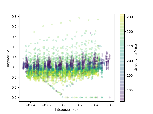
And here's a much larger set of 25,000 observations with a wider mix of strikes and moneyness:



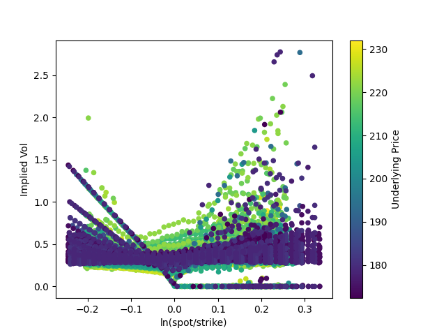
There are always some data points that don't fit the model. Here, I have set their implied volatility to zero (in the Black-Scholes graphs, I just removed them); in general, the chart seems to get wilder as moneyness increases and we begin to deal with deep in-the-money calls. Unsurprisingly, they also cluster around expiration. (There aren't as many of these outliers as it seems; if you lower the opacity of each point, they will barely be visible.)

Finally, here's a volatility surface of the above:



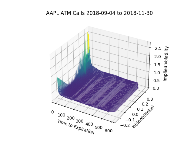
It looks pretty similar to the same surface given to us by Black-Scholes, with the same smile-shape as the option approaches expiration. This is to be expected; and comparing the Cox-Ross-Rubenstein surface to the Black-Scholes surface for the same data set is a pretty good sanity check!